Testing the webpy python module.

Today I wrote about another python module named web.py.
The reasons I start this tutorial come from google page of SDK for App Engine.
The Google come with these options of the following frameworks can be used with Python programming language:

• Flask;
• Django;
• Pyramid;
• Bottle;
• web.py
• Tornado

I started in the past to learn and use Django and I tested with Flask and Bottle and today is web.py python module.
First, about this python module I can tell you is a simple web framework and comes with a web.py slogan:
Think about the ideal way to write a web app. Write the code to make it happen.

C:\Python364\Scripts>pip install web.py==0.40-dev1
Collecting web.py==0.40-dev1
  Downloading https://files.pythonhosted.org/packages/db/a5/8dfacc190908f9876632
69a92efa682175c377e3f7eab84ed0a89c963b47/web.py-0.40.dev1.tar.gz (117kB)
    100% |████████████████████████████████| 122kB 936kB/s
Building wheels for collected packages: web.py
  Building wheel for web.py (setup.py) ... done
  Stored in directory: C:\Users\catafest\AppData\Local\pip\Cache\wheels\1b\15\12
\4fd91f5ed7e3c8aae085050cce83f72b7ca4f463bf3e67d2b7
Successfully built web.py
Installing collected packages: web.py
Successfully installed web.py-0.40.dev1

Let's test the example from the official website:

C:\Python364>python.exe
Python 3.6.4 (v3.6.4:d48eceb, Dec 19 2017, 06:54:40) [MSC v.1900 64 bit (AMD64)]
 on win32
Type "help", "copyright", "credits" or "license" for more information.
>>> import web
>>>
... urls = (
...     '/(.*)', 'hello'
... )
>>> app = web.application(urls, globals())
>>>
>>> class hello:
...     def GET(self, name):
...         if not name:
...             name = 'World'
...         return 'Hello, ' + name + '!'
...
>>> if __name__ == "__main__":
...     app.run()
...
http://0.0.0.0:8080/
127.0.0.1:50542 - - [27/Jan/2019 07:30:28] "HTTP/1.1 GET /" - 200 OK
127.0.0.1:50542 - - [27/Jan/2019 07:30:28] "HTTP/1.1 GET /favicon.ico" - 200 OK

The server starts at 0.0.0.0 (invalid address) and can see the result at 127.0.0.1:8080.

Detect nudity with nudepy python module.

Today I tested another python module named nudepy.
You can find it here.
This python module is a port of nude.js to Python.
Let's start the tutorial with the installation:

C:\Python364\Scripts>cd ..

C:\Python364>cd Scripts

C:\Python364\Scripts>pip install nudepy
Requirement already satisfied: nudepy in c:\python364\lib\site-packages (0.4)
Requirement already satisfied: pillow in c:\python364\lib\site-packages (from nu
depy) (5.3.0)

To test this python module, I used four images with the idea of a nude image
This image is the result of all images of the test.

This image files are named:

• test_nude_001.jpg
• test_nude_002.jpg
• test_nude_003.jpg
• test_nude_004.jpg

Let's see the script:

# for select jpeg files
import os, fnmatch
# import nude python module
import nude
from nude import Nude
#
nude_jpegs=fnmatch.filter(os.listdir('.'), '*nude*.jpg')
print(nude_jpegs)
for found_file in nude_jpegs:
    print (found_file)
    print("Nude file: ",nude.is_nude(str(found_file)))
    n = Nude(str(found_file))
    n.parse()
    print("and test result: ", n.result, n.inspect())
    print("====================")

The result of the output script is this:

C:\Python364>python.exe test_nude.py
['test_nude_001.jpg', 'test_nude_002.jpg', 'test_nude_003.jpg', 'test_nude_004.j
pg']
test_nude_001.jpg
Nude file:  False
and test result:  False #
====================
test_nude_002.jpg
Nude file:  False
and test result:  False #
====================
test_nude_003.jpg
Nude file:  False
and test result:  False #
====================
test_nude_004.jpg
Nude file:  True
and test result:  True #
====================

Using LibROSA python module.

This python module named LibROSA is a python package for music and audio analysis and provides the building blocks necessary to create music information retrieval systems.

C:\Python364>cd Scripts
C:\Python364\Scripts>pip install librosa
Collecting librosa
...
Successfully installed audioread-2.1.6 joblib-0.13.0 librosa-0.6.2 llvmlite-0.26.0 numba-0.41.0 resampy-0.2.1 
scikit-learn-0.20.2

Let's create one waveform and a spectrogram with this python module.
The waveform (for sound) the term describes a depiction of the pattern of sound pressure variation (or amplitude) in the time domain.
A spectrogram (known also like sonographs, voiceprints, or voicegrams) is a visual representation of the spectrum of frequencies of sound or other signals as they vary with time.
I used a free WAV file sound from here.
The result of the waveform and spectrogram for that audio file is shown into next screenshots:


My example show first the waveform and you need to close the it to see the spectrogram.
Let's see the source code of this example:

import librosa
import librosa.display
import matplotlib.pyplot as plt
plt.figure(figsize=(14, 5))
path = "merry_christmas.wav"
out,samples = librosa.load(path)
print(out.shape, samples)
librosa.display.waveplot(out, sr=samples)
plt.show()
stft_array = librosa.stft(out)
stft_array_db = librosa.amplitude_to_db(abs(stft_array))
librosa.display.specshow(stft_array_db,sr=samples,x_axis='time', y_axis='hz')
plt.colorbar()
plt.show()

Using python modules: mayavi and moviepy - part 001.

This is a simple example with two modules named: mayavi and moviepy.
Let's see the introduction of these python modules:
Mayavi2 is a general purpose, cross-platform tool for 3-D scientific data visualization. Its features include:

• Visualization of scalar, vector and tensor data in 2 and 3 dimensions.
• Easy scriptability using Python.
• Easy extendibility via custom sources, modules, and data filters.
• Reading several file formats: VTK (legacy and XML), PLOT3D, etc.
• Saving of visualizations.
• Saving rendered visualization in a variety of image formats.
• Convenient functionality for rapid scientific plotting via mlab

MoviePy is a Python module for video editing, which can be used for basic operations (like cuts, concatenations, title insertions), video compositing (a.k.a. non-linear editing), video processing, or to create advanced effects. It can read and write the most common video formats, including GIF.
The installation with pip3.6 tool:

C:\Python364\Scripts>pip3.6.exe install mayavi
Requirement already satisfied: mayavi in c:\python364\lib\site-packages (4.6.2)
...
C:\Python364\Scripts>pip3.6.exe install moviepy
Collecting moviepy
...
Installing collected packages: tqdm, moviepy
Successfully installed moviepy-0.2.3.5 tqdm-4.28.1

Let's create a simple example with these python modules.
First example:

C:\Python364>python.exe
Python 3.6.4 (v3.6.4:d48eceb, Dec 19 2017, 06:54:40) [MSC v.1900 64 bit (AMD64)]
 on win32
Type "help", "copyright", "credits" or "license" for more information.
>>> import mayavi.mlab as mlab
>>> f = mlab.gcf()
>>> f.scene._lift()
>>>

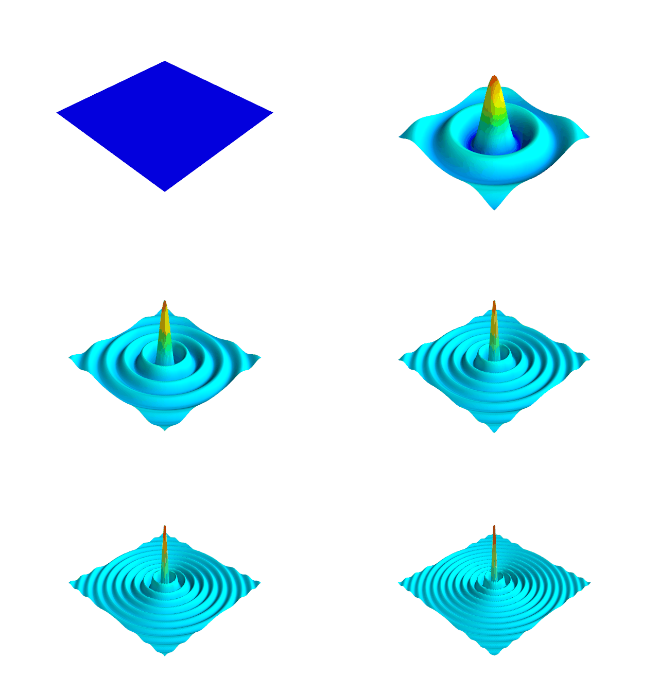
I choose the most common filter math function: the sinc function, known as sine cardinal:
In signal processing, a sinc filter is an idealized filter that removes all frequency components above a given cutoff frequency, without affecting lower frequencies, and has linear phase response. The filter's impulse response is a sinc function in the time domain, and its frequency response is a rectangular function.
I create the example to show you a sinc function by time.
This is my output (is not the result of the frequency response of the Fourier transform of the rectangular function).

Let's see the source code:

# import python modules
import numpy as np
import mayavi.mlab as mlab
import moviepy.editor as mpy
# duration of the animation in seconds 
duration= 2
# create the grid of points for x and y
x, y = np.mgrid[-30:30:100j, -30:30:100j]
# create the size figure
fig = mlab.figure(size=(640,480), bgcolor=(1,1,1))
# create the plane surface
r = np.sqrt(x**2 + y**2)
# this fix issue https://github.com/enthought/mayavi/issues/702
fig = mlab.gcf()
fig.scene._lift()
# create all frames 
def make_frame(t):
    # clear the area 
    mlab.clf()
    #blend surface by z over time t step is 0.05
    z = np.sin(r*t)/r
    # create surface 
    mlab.surf(z, warp_scale='auto')
    return mlab.screenshot(antialiased=True)
# create animation movie clip
animation = mpy.VideoClip(make_frame,duration=duration)
# write file like a GIF 
animation.write_gif("sinc.gif", fps=20)

Python Qt5 : the most simple QTreeWidget - part 001.

The QTreeWidget is more complex in order to accomplish a simple development issue.
Today, I will show you how is the first step to start it.
This simple example will follow these goals:

• create a simple QTreeWidget;
• use the most simple way to do that;
• do not use the class object;
• show files and folders;

The example do not have any feature for and show my C drive:

• filter, sort and drag and drop;

The result of this example:

Using pytorch - the final of story.

Let's continue our story with the child and the gift.
The child saw the gift and his first thought was the desire to know.
The basic forming unit of a neural network is a perceptron.
He saw that he was not too big and his eyes lit up.
To compute the output will multiply input with respective weights and compare with a threshold value.
Each perceptron also has a bias which can be thought of as how much flexible the perceptron is.
This process is of evolving a perceptron to what a now called an artificial neuron.
The next step is the artificial network and is all artificial neuron and edges between.
He touched him in the corners and put his hand on his surface.
The activation function is mostly used to make a non-linear transformation which allows us to fit nonlinear hypotheses or to estimate the complex functions.
He began to understand that he had a special and complex form.
This artificial network is built from start to end from:

• Input Layer an X as an input matrix;
• Hidden Layers a matrix dot product of input and weights assigned to edges between the input and hidden layer, then add biases of the hidden layer neurons to respective inputs and use this to update all weights at the output and hidden layer to use update biases at the output and hidden layer.
• Output Layer an y as an output matrix;

Without too much thoughts he began to break out of the gift in the order in which he touched it.
This weight and bias of the updating process are known as back propagation.
To computed the output and this process is known as forward propagation.
Several moves were enough to complete the opening of the gift.
He looked and understood that the size of the gift is smaller, but the gift was thankful to him.
This forward and back propagation iteration is known as one training iteration named epoch.
The next example I created from an old example I saw on the internet and is the most simple way to show you the steps from this last part of the story:

##use an neural network in pytorch
import torch

#an input array
X = torch.Tensor([[1,0,1],[0,1,1],[0,1,0]])

#the output
y = torch.Tensor([[1],[1],[0]])

#the Sigmoid Function
def sigmoid (x):
  return 1/(1 + torch.exp(-x))

#the derivative of Sigmoid Function
def derivatives_sigmoid(x):
  return x * (1 - x)

#set the variable initialization
epoch=1000 #training iterations is epoch
lr=0.1 #learning rate value
inputlayer_neurons = X.shape[1] #number of features in data set
hiddenlayer_neurons = 3 #number of hidden layers neurons
output_neurons = 1 #number of neurons at output layer

#weight and bias initialization
wh=torch.randn(inputlayer_neurons, hiddenlayer_neurons).type(torch.FloatTensor)
print("weigt = ", wh)
bh=torch.randn(1, hiddenlayer_neurons).type(torch.FloatTensor)
print("bias = ", bh)
wout=torch.randn(hiddenlayer_neurons, output_neurons)
print("wout = ", wout)
bout=torch.randn(1, output_neurons)
print("bout = ", bout)

for i in range(epoch):

  #Forward Propogation
  hidden_layer_input1 = torch.mm(X, wh)
  hidden_layer_input = hidden_layer_input1 + bh
  hidden_layer_activations = sigmoid(hidden_layer_input)
 
  output_layer_input1 = torch.mm(hidden_layer_activations, wout)
  output_layer_input = output_layer_input1 + bout
  output = sigmoid(output_layer_input1)

  #Backpropagation
  E = y-output
  slope_output_layer = derivatives_sigmoid(output)
  slope_hidden_layer = derivatives_sigmoid(hidden_layer_activations)
  d_output = E * slope_output_layer
  Error_at_hidden_layer = torch.mm(d_output, wout.t())
  d_hiddenlayer = Error_at_hidden_layer * slope_hidden_layer
  wout += torch.mm(hidden_layer_activations.t(), d_output) *lr
  bout += d_output.sum() *lr
  wh += torch.mm(X.t(), d_hiddenlayer) *lr
  bh += d_output.sum() *lr
 
print('actual :\n', y, '\n')
print('predicted :\n', output)

The result is for 100 and 1000 epoch value and show us how close is the actual input (1,1,0) to the predicted results.
See also the weight and bias initialization of the artificial network is created random by torch.randn.
If I added this in my story it would sound like this:
The child's thoughts began to flinch in wanting to finish faster and find the gift.

C:\Python364>python.exe pytorch_test_002.py
weigt =  tensor([[-0.9364,  0.4214,  0.2473],
        [-1.0382,  2.0838, -1.2670],
        [ 1.2821, -0.7776, -1.8969]])
bias =  tensor([[-0.3604, -0.8943,  0.3786]])
wout =  tensor([[-0.5408],
        [ 1.3174],
        [-0.7556]])
bout =  tensor([[-0.4228]])
actual :
 tensor([[1.],
        [1.],
        [0.]])

predicted :
 tensor([[0.5903],
        [0.6910],
        [0.6168]])

C:\Python364>python.exe pytorch_test_002.py
weigt =  tensor([[ 1.2993,  1.5142, -1.6325],
        [ 0.0621, -0.5370,  0.1480],
        [ 1.5673, -0.2273, -0.3698]])
bias =  tensor([[-2.0730, -1.2494,  0.2484]])
wout =  tensor([[ 0.6642],
        [ 1.6692],
        [-0.4087]])
bout =  tensor([[0.3340]])
actual :
 tensor([[1.],
        [1.],
        [0.]])

predicted :
 tensor([[0.9417],
        [0.8510],
        [0.2364]])

Python Qt5 : simple draw with QPainter.

Using the QPainter is more complex than a simple example.
I try to create a simple example in order to have a good look at how can be used.
The main goal was to understand how can have the basic elements of QPainter.
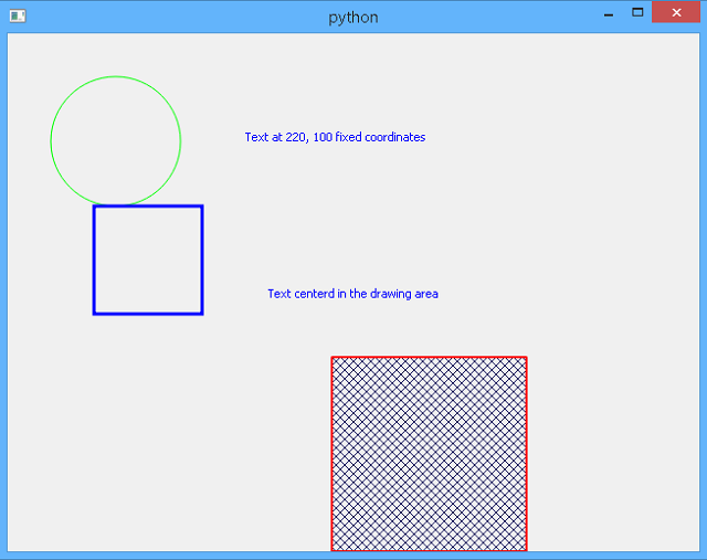
The result of my example is this:

Here is my example with all commented lines for a good approach:

import sys 
from PyQt5 import QtGui, QtWidgets 
from PyQt5.QtGui import QPainter, QBrush, QColor
from PyQt5.QtCore import Qt, QPoint 
class My_QPainter(QtWidgets.QWidget): 
    def paintEvent(self, event): 
        # create custom QPainter
        my_painter = QtGui.QPainter() 
        # start and set my_painter
        my_painter.begin(self) 
        my_painter.setRenderHint(my_painter.TextAntialiasing, True)
        my_painter.setRenderHint(my_painter.Antialiasing, True)
        #set color for pen by RGB
        my_painter.setPen(QtGui.QColor(0,0,255)) 
        # draw a text on fixed coordinates
        my_painter.drawText(220,100, "Text at 220, 100 fixed coordinates") 
        # draw a text in the centre of my_painter   
        my_painter.drawText(event.rect(), Qt.AlignCenter, "Text centerd in the drawing area") 
        #set color for pen by Qt color  
        my_painter.setPen(QtGui.QPen(Qt.green, 1)) 
        # draw a ellipse
        my_painter.drawEllipse(QPoint(100,100),60,60) 
        # set color for pen by property
        my_painter.setPen(QtGui.QPen(Qt.blue, 3, join = Qt.MiterJoin)) 
        # draw a rectangle
        my_painter.drawRect(80,160,100,100) 
        # set color for pen by Qt color 
        my_painter.setPen(QtGui.QPen(Qt.red, 2))
        # set brush 
        my_brush = QBrush(QColor(33, 33, 100, 255), Qt.DiagCrossPattern)
        my_painter.setBrush(my_brush)
        # draw a rectangle and fill with the brush 
        my_painter.drawRect(300, 300,180, 180)
        my_painter.end() 
# create application  
app = QtWidgets.QApplication(sys.argv) 
# create the window application from class
window = My_QPainter() 
# show the window
window.show() 
# default exit 
sys.exit(app.exec_())

Python 3.6.4 : Learning OpenCV - centroids.

Today I was a little lazy.
I studied a little on the internet.
The last aspect was related to centroids.
An example I studied before TV news was from this webpage.
About centroid you can read here.
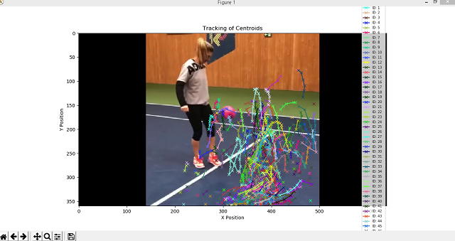
The result of the source code from a video with Simona Halep.

Python Qt5 : complex QML file.

Today, I will show you how to have a more complex custom application with PyQt5 and QML file.
You need to create into your python folder a new folder named QMLCustom.
Into this file create two python files named: __init__.py and QMLCustom.py.
The __init__ will be an empty file.
Into your python folder installation (where you create the QMLCustom folder), create a new QML_custom.qml file.
The QML_custom.qml file will have this:

import QtQuick 2.0
import SDK 1.0
import QtQuick.Layouts 1.1

Rectangle {
    id: appwnd
    visible: true
    width: 640
    height: 480

    property int columns : 2
    property int rows : 2

    Rectangle {
        anchors.fill: parent
        color: "#00f"
    }

    GridView {
        id: grid
        anchors.fill: parent
        cellWidth: Math.max(width/2, height/2);
        cellHeight: Math.max(width/2, height/2)
        model: dashModel
        delegate : Rectangle {
            Layout.alignment: Layout.Center
            width: grid.cellWidth
            height: grid.cellHeight
            color: "#0ff"
            border.color: "#fff"
            border.width: 10

            Text {
                id: name
                anchors.horizontalCenter: parent.horizontalCenter
                anchors.bottom: parent.bottom
                anchors.leftMargin:15
                anchors.topMargin: 15
                width: parent.width 
                height: parent.height
                textFont {
                    family: "Halvetica"
                    italic: false
                    pointSize:20
                }
                suffixText: suffix
            }

        }
        onWidthChanged: {
            grid.cellWidth = grid.width/appwnd.columns;
        }

        onHeightChanged: {
            grid.cellHeight = grid.height/appwnd.rows
        }
    }

    ListModel {
        id: dashModel
        ListElement {
            tagName: "Text"
            suffix: "First text"
        }
        ListElement {
            tagName: "Text"
            suffix: "Next text"
        }         
    }
} 

If you read this you will see the qml type file has two imports and a text.
The imports are used to load it and the text file is used to describe what we need.
In this case is created a Rectangle, GridView and one ListModel with two ListElement.
All of this part will be a link to the QMLCustom.py file.
For example: follow the suffixText from qml file suffixText: suffix into QMLCustom.py file (decorator def suffixText(self, text)).
Into the QMLCustom folder you need to fill the QMLCustom.py with this:

import PyQt5
from PyQt5.QtCore import *
from PyQt5.QtGui import *
from PyQt5.QtWidgets import *
from PyQt5.QtCore import pyqtProperty, pyqtSignal, pyqtSlot
from PyQt5.QtQuick import QQuickPaintedItem, QQuickItem
from PyQt5.QtGui import QPainter
from PyQt5 import QtCore

class QMLCustom(QQuickPaintedItem):
    #
    class DialType():
        FullDial = 0
        MinToMax = 1
        NoDial = 2
    #
    sizeChanged = pyqtSignal()
    valueChanged = pyqtSignal()
    #
    backgroundColorChanged = pyqtSignal()
    #
    textColorChanged = pyqtSignal()
    suffixTextChanged = pyqtSignal()
    showTextChanged = pyqtSignal()
    textFontChanged = pyqtSignal()

    def __init__(self, parent=None):
        super(QMLCustom, self).__init__(parent)

        self.setWidth(100)
        self.setHeight(100)
        self.setSmooth(True)
        self.setAntialiasing(True)

        self._Size = 100
        self._DialWidth = 15
        self._SuffixText = ""
        self._BackgroundColor = Qt.transparent
        self._TextColor = QColor(0, 0, 0)
        self._ShowText = True
        self._TextFont = QFont()

    def paint(self, painter):
        painter.save()

        size = min(self.width(), self.height())       
        self.setWidth(size)
        self.setHeight(size)
        rect = QRectF(0, 0, self.width(), self.height()) 
        painter.setRenderHint(QPainter.Antialiasing)
        
        painter.restore()

        painter.save()
        painter.setFont(self._TextFont)
        offset = self._DialWidth / 2
        if self._ShowText:
            painter.drawText(rect.adjusted(offset, offset, -offset, -offset), Qt.AlignCenter, self._SuffixText)
        else:
            painter.drawText(rect.adjusted(offset, offset, -offset, -offset), Qt.AlignCenter, self._SuffixText)
        painter.restore()

    @QtCore.pyqtProperty(str, notify=sizeChanged)
    def size(self):
        return self._Size

    @size.setter
    def size(self, size):
        if self._Size == size:
            return
        self._Size = size
        self.sizeChanged.emit()

    @QtCore.pyqtProperty(float, notify=valueChanged)
    def value(self):
        return self._Value

    @value.setter
    def value(self, value):
        if self._Value == value:
            return
        self._Value = value
        self.valueChanged.emit()


    @QtCore.pyqtProperty(QColor, notify=backgroundColorChanged)
    def backgroundColor(self):
        return self._BackgroundColor

    @backgroundColor.setter
    def backgroundColor(self, color):
        if self._BackgroundColor == color:
            return
        self._BackgroundColor = color
        self.backgroundColorChanged.emit()


    @QtCore.pyqtProperty(QColor, notify=textColorChanged)
    def textColor(self):
        return self._TextColor

    @textColor.setter
    def textColor(self, color):
        if self._TextColor == color:
            return
        self._TextColor = color
        self.textColorChanged.emit()  

    @QtCore.pyqtProperty(str, notify=suffixTextChanged)
    def suffixText(self):
        return self._SuffixText

    @suffixText.setter
    def suffixText(self, text):
        if self._SuffixText == text:
            return
        self._SuffixText = text
        self.suffixTextChanged.emit()

    @QtCore.pyqtProperty(str, notify=showTextChanged)
    def showText(self):
        return self._ShowText

    @showText.setter
    def showText(self, show):
        if self._ShowText == show:
            return
        self._ShowText = show


    @QtCore.pyqtProperty(QFont, notify=textFontChanged)
    def textFont(self):
        return self._TextFont

    @textFont.setter
    def textFont(self, font):
        if self._TextFont == font:
            return
        self._TextFont = font
        self.textFontChanged.emit()

This is a base python module that allows you to use the qml file and show it into your application.
The QMLCustom.py use a class (with pyqtSignal and paint to link all data with decorators) to be used into your application.
This can be a little difficult to follow but if you deal with a tool like QtCreator editor you will understand how this integrated GUI layout and forms designer with this script.
The last part is more simple and is the application.
This script uses both the custom python module QMLCustom and the qml file.
Create a python file into your folder python installation fill with the next script and run it:

import sys
import os
import subprocess

from QMLCustom.QMLCustom import QMLCustom

from PyQt5.QtCore import QUrl, Qt, QObject, pyqtSignal, pyqtSlot
from PyQt5.QtGui import QGuiApplication, QCursor
from PyQt5.QtQuick import QQuickView
from PyQt5.QtQml import qmlRegisterType
from OpenGL import GLU

class App(QGuiApplication):
 def __init__(self, argv):
  super(App, self).__init__(argv)

if __name__ == '__main__':
 try:
  app = App(sys.argv)
  
  qmlRegisterType(QMLCustom, "SDK", 1,0, "Text")

  view = QQuickView()
  ctxt = view.rootContext()
  view.setSource(QUrl("QML_custom.qml"))
  view.show()
  ret = app.exec_()

 except Exception as e:
  print (e)

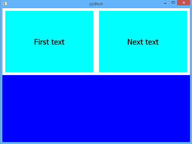
The result is this:

Python Qt5 : application with QML file.

The PyQt5 includes QML as a means of declaratively describing a user interface and is possible to write complete standalone QML applications.
Using QML file is different from the versions PyQt5 and old PyQt4.
Using this type of application can let you solve custom and style application.
I create a simple example but can create your python module with a class with new type of style.
This can be used with qmlRegisterType for your new python class type.
Let's see the example:
The main python file:

from PyQt5.QtNetwork import *
from PyQt5.QtQml import *
from PyQt5.QtWidgets import *
from PyQt5.QtCore import *

class MainWin(object):
    def __init__(self):
        self.eng = QQmlApplicationEngine()
        self.eng.load('win.qml')
        win = self.eng.rootObjects()[0]   
        win.show()

if __name__ == '__main__':
    import sys
    App = QApplication(sys.argv)
    Win = MainWin()
    sys.exit(App.exec_())

The QML file:

import QtQuick 2.2
import QtQuick.Controls 1.0
ApplicationWindow {
    id: main
    width: 640
    height: 480
    color: 'blue'
 }

The result is a blue window.

Using pytorch - another way.

Yes. I used pytorch and is working well. Is not perfect the GitHub come every day with a full stack of issues.
Let's continue this series with another step: torchvision.
If you take a closer look at that gift, you will see that it comes with a special label that can really help us.
This label is a named torchvision.
The torchvision python module is a package consists of popular datasets, model architectures, and common image transformations for computer vision.
Most operations pass through filters and date already recognized.

• torchvision.datasets: (MNIST,Fashion-MNIST,EMNIST,COCO,LSUN,ImageFolder,DatasetFolder,Imagenet-12,CIFAR,STL10,SVHN,PhotoTour,SBU,Flickr,VOC)
• torchvision.models: (Alexnet,VGG,ResNet,SqueezeNet,DenseNet,Inception v3)
• torchvision.transforms: (Transforms on PIL Image,Transforms on torch.*Tensor,Conversion Transforms,Generic Transforms,Functional Transforms)
• torchvision.utils

This part of the gift help you to load and prepare dataset but into certain order.
Using this special label, we will be able to use the gift-breaking information.
Let's see the example:

C:\Python364>python.exe
Python 3.6.4 (v3.6.4:d48eceb, Dec 19 2017, 06:54:40) [MSC v.1900 64 bit (AMD64)]
 on win32
Type "help", "copyright", "credits" or "license" for more information.
>>> import torchvision
>>> import torchvision.transforms as transforms
>>> transform = transforms.Compose(
...     [transforms.ToTensor(),
...      transforms.Normalize((0.5, 0.5, 0.5), (0.5, 0.5, 0.5))])
>>> trainset = torchvision.datasets.CIFAR10(root='./data', train=True,download=T
rue, transform=transform)
Downloading https://www.cs.toronto.edu/~kriz/cifar-10-python.tar.gz to ./data\ci
far-10-python.tar.gz

You will ask me: How is this special gift label linked?
In this way:

>>> import torch
>>> trainloader = torch.utils.data.DataLoader(trainset, batch_size=4,shuffle=Tru
e, num_workers=2)

Let's take a closer look at the information in the special label.

>>> print(trainset)
Dataset CIFAR10
    Number of datapoints: 50000
    Split: train
    Root Location: ./data
    Transforms (if any): Compose(
                             ToTensor()
                             Normalize(mean=(0.5, 0.5, 0.5), std=(0.5, 0.5, 0.5)
)
                         )
    Target Transforms (if any): None
>>> print(dir(trainset))
['__add__', '__class__', '__delattr__', '__dict__', '__dir__', '__doc__', '__eq_
_', '__format__', '__ge__', '__getattribute__', '__getitem__', '__gt__', '__hash
__', '__init__', '__init_subclass__', '__le__', '__len__', '__lt__', '__module__
', '__ne__', '__new__', '__reduce__', '__reduce_ex__', '__repr__', '__setattr__'
, '__sizeof__', '__str__', '__subclasshook__', '__weakref__', '_check_integrity'
, 'base_folder', 'download', 'filename', 'root', 'target_transform', 'test_list'
, 'tgz_md5', 'train', 'train_data', 'train_labels', 'train_list', 'transform', '
url']

Let's look more closely at the information that can be used by the gift with the special label.

>>> print(trainloader)

>>> print(dir(trainloader))
['_DataLoader__initialized', '__class__', '__delattr__', '__dict__', '__dir__',
'__doc__', '__eq__', '__format__', '__ge__', '__getattribute__', '__gt__', '__ha
sh__', '__init__', '__init_subclass__', '__iter__', '__le__', '__len__', '__lt__
', '__module__', '__ne__', '__new__', '__reduce__', '__reduce_ex__', '__repr__',
 '__setattr__', '__sizeof__', '__str__', '__subclasshook__', '__weakref__', 'bat
ch_sampler', 'batch_size', 'collate_fn', 'dataset', 'drop_last', 'num_workers',
'pin_memory', 'sampler', 'timeout', 'worker_init_fn']

Beware, CIFAR10 is just one of the training databases.
About the CIFAR-10 dataset, that consists of 60,000 32x32 color images in 10 classes, with 6,000 images per class.
There are 50,000 training images (5,000 per class) and 10,000 test images.

Fix errors when write files.

The python is a very versatile programming language.
The tutorial for today is about:

• check the type of variables;
• see the list error of writelines with the list output;
• fix errors for writelines;

One good example for some errors can be this:

>>> file.writelines(paragraphs)
Traceback (most recent call last):
  File "", line 1, in 
TypeError: a bytes-like object is required, not 'str'
>>> file.writelines(paragraphs.decode('utf-8'))
Traceback (most recent call last):
  File "", line 1, in 
AttributeError: 'list' object has no attribute 'decode'

Is a common issue for list and writing file.
The result of paragraphs is a list, see:

>>> type(paragraphs)

The list can be write with te writelines into the file like this:

>>> file = open("out.txt","wb")
>>> file.writelines([word.encode('utf-8') for word in paragraphs])

The file is a open file variable and the paragraphs is a list.

Using pytorch - a simpler perspective.

Suppose this module PyTorch is a data extravagance circuit that allows us to filter information several times, and we can decide each time we decide the final result.
A simpler perspective of how to work with PyTorch can be explained by a simple example.
It's like a Christmas baby (PyTorch) that opens a multi-packed gift until it gets the final product - the desired gift.
The opening operations of the package involve smart moves called: forward and backward passes.
The child's feedback can be called: loss and backpropagate.
In this case, the child will try to remove from his package until he is satisfied and will not be lost (loss and backpropagate functions).
To compute the backward pass for a gradient and every time we backpropagate the gradient from a variable, the gradient is accumulative instead of being reset and replaced (most of networks designs call backward multiple times).
PyTorch comes with many loss functions.
Most of examples code create a mean square error loss function and later backpropagate the gradients based on the loss.
Will you ask me if the gift is shaped? I can tell you that the gift can contain from Verge à Saint-Nicolas (unidimensional) to complex (multidimensional) structures - the most simplistic and worn out is the square one (two-dimensional matrix).
This gift is packed with magic in mathematical functions which allows the child to understand what is in the gift.
But the child is more special. He recognizes forms (matrices, shapes, simple formulas) and this allows him to open parts of the gift.
El poate roti acesta parti din cadou (mm).
The mm is a matrix multiplication.
He can see the corners he can get from the gift.
ReLU stands for "rectified linear unit" and is a type of activation function.
Mathematically, it is defined as y = max(0, x).
He can see which parts of the gift are bigger or smaller so he can understand the gift.
This clamp function clamps all elements in input into the returns[ min, max ] and returns a resulting tensor:
The clamp should only affect gradients for values outside the min and max range.
The pow function power with the exponent.
The clone returns a copy of the self tensor. The copy has the same size and data type as self.
A common example is: clamp(min=0) is exactly ReLU().
PyTorch provides ReLU and its variants through the torch.nn module.
If you run the program to look at the output, you will understand that the child has only five operations left and is already pleased with the way the gift result.
The source code is based on one example from here:

import torch 
dtype = torch.float
device = torch.device("cpu")
batch,input,hidden,output = 2,10,2,5
x = torch.randn(batch,input,device=device,dtype=dtype)
y = torch.randn(hidden,output,device=device,dtype=dtype)
w1 = torch.randn(input,hidden,device=device,dtype=dtype)
w2 = torch.randn(hidden,output,device=device,dtype=dtype)

l_r = 1e-6
for t in range(5):
 h = x.mm(w1)
 h_r = h.clamp(min=0)
 y_p = h_r.mm(w2)
 loss = (y_p - y).pow(2).sum().item()
 print("t=",t,"loss=",loss,"\n")
 g_y_p = 2.0 * (y_p -y)
 g_w2 = h_r.t().mm(g_y_p)
 g_h_r = g_y_p.mm(w2.t())
 g_h = g_h_r.clone()
 g_h[h<0 -="l_r" 0="" g_w1="" g_w2="" n="" print="" w1=",w1," w2=",w2,">

The child's result after five operations.

...
t= 4 loss= 25.40263557434082

w1= tensor([[ 1.5933,  0.3818],
        [-1.0043, -1.3362],
        [ 0.5841, -1.9811],
        [ 2.3483,  0.5748],
        [ 0.5904, -0.2521],
        [-0.6612,  2.7945],
        [ 0.4841, -0.5894],
        [-1.4434, -0.1421],
        [-1.2712, -1.4269],
        [ 0.7929,  0.2040]]) w2= tensor([[ 1.7389,  0.4337,  0.4557,  1.3704,  0
.3819],
        [ 0.2937,  0.0212, -0.4604, -1.0564, -1.5403]])