analitics

Pages

Saturday, October 10, 2020

Python 3.9.0 : Introduction to release 3.9.0.

This is a short introduction to release 3.9.0. 
Five days ago, a new release of version 3.9 appeared with a series of improvements and new python packages, see the official website
You can install easily on Fedora 32 with dnf tool.
[root@desk mythcat]# dnf install  python39.x86_64
...
Installing:
 python39                x86_64                3.9.0-1.fc32
...
Installed:
  python39-3.9.0-1.fc32.x86_64                                                                             

Complete!
A new article written about this release shows some of the advantages of this programming language, you can read it here
You can run easily with this command;
[root@desk mythcat]# python3.9
Python 3.9.0 (default, Oct  6 2020, 00:00:00) 
[GCC 10.2.1 20200723 (Red Hat 10.2.1-1)] on linux
Type "help", "copyright", "credits" or "license" for more information. 
You can configure python with this command, see an example:
[root@desk mythcat]# python3.9-x86_64-config --libs 
 -lcrypt -lpthread -ldl  -lutil -lm -lm 
This release of Python 3.9 uses a new parser, based on parsing expression grammar (PEG) instead of LL(1) know as LL parser (Left-to-right, Leftmost derivation). PEG parsers are more powerful than LL(1) parsers and avoid the need for special hacks. This the same abstract syntax tree (AST) as the old LL(1) parser. The PEG parser is the default, but you can run your program using the old parser, see the next example:
[mythcat@desk ~]$ python3.9 -X oldparser my_script_name.py
...
One of the most important improvements for me is PEP 614 -- Relaxing Grammar Restrictions On Decorators. In Python 3.9, these restrictions are lifted and you can now use any expression. 
For example including one accessing items in a dictionary, like this simple example:

buttons = {
  "hello": QPushButton("hello word!"),
  "bye": QPushButton("bye word!"),
  "buy": QPushButton("buy!!"),
}
...
@buttons["hello"].clicked.connect
def speak_hello():
... 
Yes, comes with another Python Enhancement Proposals - PEP 615 with support for the IANA Time Zone Database in the Standard Library. This acronym is similar to I.A.N.A known as the Internet Assigned Numbers Authority, but it is not the same. 
In this case, the zoneinfo module provides a concrete time zone implementation to support the IANA time zone database. 
This support contains code and data that represent the history of local time for many representative locations around the globe. Many features for math, strings, union operator for the dictionary, HTTP codes, and more. 
Completion of variable and module names is automatically enabled at interpreter startup so that the Tab key invokes the completion function. 
You can see a simple example with zoneinfo python module and completion feature.
[mythcat@desk ~]$ python3.9
Python 3.9.0 (default, Oct  6 2020, 00:00:00) 
[GCC 10.2.1 20200723 (Red Hat 10.2.1-1)] on linux
Type "help", "copyright", "credits" or "license" for more information.
>>> from zoneinfo import ZoneInfo
>>> import zoneinfo
>>> zoneinfo.available_timezones()
{'Hongkong', 'America/Iqaluit', 'America/Indianapolis', 'America/Louisville', 'America/New_York', 
'America/Mazatlan', 'Australia/Yancowinna', 'Africa/Ndjamena', 'Portugal', 'Africa/Bujumbura', 
'America/Rosario', 'America/Antigua','America/Indiana/Tell_City', 'America/Managua', 
'Europe/Paris', 'Europe/Oslo', 
...
>>> tz = ZoneInfo("Europe/Bucharest")
>>> tz.
tz.clear_cache(  tz.from_file(    tz.key           tz.tzname(       
tz.dst(          tz.fromutc(      tz.no_cache(     tz.utcoffset(    
>>> tz. 
On my desktop I got this result:
[mythcat@desk ~]$ python var_access_benchmark.py 
Variable and attribute read access:
   6.0 ns	read_local
   6.5 ns	read_nonlocal
  10.7 ns	read_global
  10.7 ns	read_builtin
  25.2 ns	read_classvar_from_class
  23.4 ns	read_classvar_from_instance
  34.3 ns	read_instancevar
  29.4 ns	read_instancevar_slots
  26.8 ns	read_namedtuple
  42.4 ns	read_boundmethod

Variable and attribute write access:
   6.6 ns	write_local
   7.0 ns	write_nonlocal
  23.3 ns	write_global
  54.1 ns	write_classvar
  46.4 ns	write_instancevar
  39.4 ns	write_instancevar_slots

Data structure read access:
  26.1 ns	read_list
  28.1 ns	read_deque
  27.5 ns	read_dict
  25.8 ns	read_strdict

Data structure write access:
  29.6 ns	write_list
  31.7 ns	write_deque
  34.4 ns	write_dict
  31.7 ns	write_strdict

Stack (or queue) operations:
  55.5 ns	list_append_pop
  49.7 ns	deque_append_pop
  51.0 ns	deque_append_popleft

Timing loop overhead:
   0.4 ns	loop_overhead

Tuesday, September 29, 2020

Python Qt5 : Use QStandardItem with Images.

This tutorial show you how to use QStandardItem with Images.

The source code is simple to understand.

import sys
from PyQt5.QtWidgets import QApplication, QMainWindow, QTreeView
from PyQt5.QtCore import  Qt
from PyQt5.QtGui import QFont, QColor, QImage, QStandardItemModel, QStandardItem

class ItemImage(QStandardItem):
    def __init__(self, txt='', image_path='', set_bold=False, color=QColor(0, 0, 0)):
        super().__init__()

        self.setEditable(False)
        self.setForeground(color)
        self.setText(txt)

        if image_path:
            image = QImage(image_path)
            self.setData(image, Qt.DecorationRole)

class MyApp(QMainWindow):
    def __init__(self):
        super().__init__()
        self.resize(1200, 1200)

        treeView = QTreeView()
        treeView.setHeaderHidden(True)
        treeView.header().setStretchLastSection(True)

        treeModel = QStandardItemModel()
        rootNode = treeModel.invisibleRootItem()

        robots = ItemImage('Robots', '', set_bold=True)

        aaa = ItemImage('aaa.jpg', 'aaa.jpg', 14)
        robots.appendRow(aaa)

        bbb = ItemImage('bbb.jpg', 'bbb.jpg', 16)
        robots.appendRow(bbb)

        robots2 = ItemImage('Robots 2', '', set_bold=False)

        aaa = ItemImage('ccc.png', 'ccc.png', 14)
        robots2.appendRow(aaa)

        bbb = ItemImage('ddd.jpg', 'ddd.jpg', 16)
        robots2.appendRow(bbb)

        rootNode.appendRow(robots)
        rootNode.appendRow(robots2)
        treeView.setModel(treeModel)
        treeView.expandAll()

        self.setCentralWidget(treeView)

app = QApplication(sys.argv)        
demo = MyApp()
demo.show()
sys.exit(app.exec_())

The result is this:

Monday, September 21, 2020

Python 3.8.5 : A sphere in Cartesian coordinates - part 001.

I like the equation of a sphere of radius R centered at the origin is given in Cartesian coordinates:

x*x + y*y + z*z = r*r

It is one of the first elements that helped me better understand mathematics and later the dynamics and theory of electromagnetic fields.

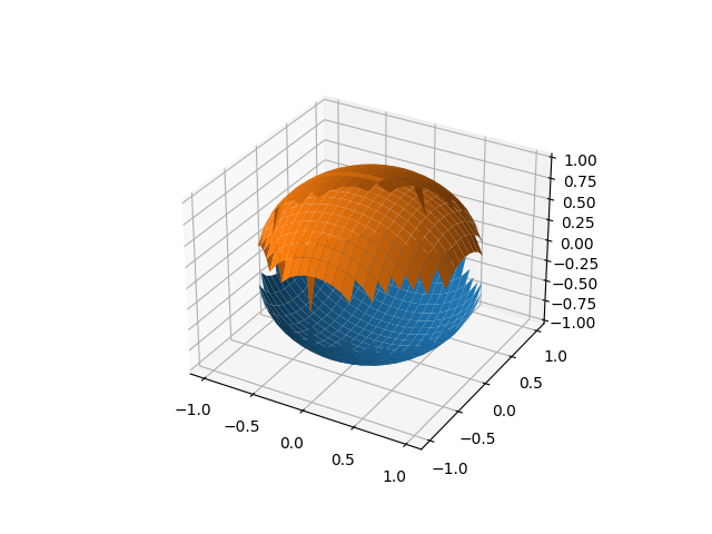
I did not find a graphical representation using python as accurately as possible without eliminating the discretion of the range from -1 and 1 and radius * radius = 1.

The main reason is the plot_surface from matplotlib python package.

This is output of my script:

[mythcat@desk ~]$ python sphere_xyz.py 
[-1.         -0.91666667 -0.83333333 -0.75       -0.66666667 -0.58333333
 -0.5        -0.41666667 -0.33333333 -0.25       -0.16666667 -0.08333333
  0.          0.08333333  0.16666667  0.25        0.33333333  0.41666667
  0.5         0.58333333  0.66666667  0.75        0.83333333  0.91666667
  1.        ]
sphere_xyz.py:7: RuntimeWarning: invalid value encountered in sqrt
  return np.sqrt(1-x**2 - y**2)
sphere_xyz.py:18: UserWarning: Z contains NaN values. This may result in rendering artifacts.
  surface1 = ax.plot_surface(X2, Y2, -Z2,rstride=1, cstride=1, linewidth=0,antialiased=True)
sphere_xyz.py:19: UserWarning: Z contains NaN values. This may result in rendering artifacts.
  surface2 = ax.plot_surface(X2, Y2, Z2,rstride=1, cstride=1, linewidth=0,antialiased=True)

The image result is this:

The source code is this:

import matplotlib.pyplot as plt
import numpy as np
from matplotlib.colors import LightSource

#@np.vectorize
def solve_Z2(x,y):
    return np.sqrt(1-x**2 - y**2)

fig = plt.figure()
ax = fig.gca(projection='3d')

xrange2 = np.linspace(-1.0, 1.0, 25)
yrange2 = np.linspace(-1.0, 1.0, 25)
print(xrange2)
X2, Y2 = np.meshgrid(xrange2, yrange2)
Z2 = solve_Z2(X2, Y2)

surface1 = ax.plot_surface(X2, Y2, -Z2,rstride=1, cstride=1, linewidth=0,antialiased=True)
surface2 = ax.plot_surface(X2, Y2, Z2,rstride=1, cstride=1, linewidth=0,antialiased=True)

plt.show()

Saturday, September 19, 2020

Python 3.8.5 : Linked List - part 001.

In computer science, a linked list is a linear collection of data elements whose order is not given by their physical placement in memory. see wikipedia.org.

In this tutorial I will show you how these linked list works and how can build with python programming language.
Let's start with some basic elements:
  • Linked List is a linear data structure;
  • Linked List are not array;
  • Linked List are not stored at a contiguous location because use pointes;
  • Each element use a linked pointe;
  • Linked List has a dynamic size;
  • Linked List use operations like insertion and deletion for each element;
  • The access to elements is sequentially;
  • Using reference to pointer foe each element needs extra memory space and is not cache friendly;

The Linked List consists of at least two parts: data and pointer to the next node.
The first element of the list is called the head.

The last node has a reference to null.
The each element named node of the list has a similar structure like Linked List: data node and pointer to the next node.
The data from Linked list is represent like a sequence.

A number of operations are required to use the Linked List.

The basic operations supported by a list can be:

  • insertion - adds an element at the beginning of the list;
  • deletion - deletes an element at the beginning of the list;
  • display - displays the complete list;
  • search - searches an element using the given key;
  • delete - deletes an element using the given key.

The Advantages of Linked List elements can be easily inserted or removed without reallocation or reorganization of the entire structure because the data items need not be stored contiguously in memory or on disk using operations.

The Linked List structure allows several ways to link nodes resulting in a number of types of Linked List:
  • Simple linked list;
  • Doubly linked list;
  • Multiply linked list;
  • Circular linked list;
  • Sentinel nodes;
  • Empty lists;
  • Hash linking;
  • List handles;
  • Combining alternatives;

Let's start with first source code for the first type of Linked List named Simple linked list.

Python 3.8.5 (default, Aug 12 2020, 00:00:00) 
[GCC 10.2.1 20200723 (Red Hat 10.2.1-1)] on linux
Type "help", "copyright", "credits" or "license" for more information.
>>> # create a node class 
>>> class Node:
...     # first initialise of the node object
...     def __init__(self, data):
...             # assign the node data 
...             self.data = data
...             # initialize next element as null
...             self.next = None
... 
>>> # create a simple linked list
>>> class Simple_LinkedList:
...     # first initialize of element named head
...     def __init__(self):
...             self.head = None
>>> # use the list 
>>> if __name__=='__main__': 
...     simple_list = Simple_LinkedList()
...     simple_list.head = Node(1)
...     second = Node(2)
...     third = Node(3)
...     #link first node with the second
...     simple_list.head.next = second
...     #link second  node with the third
...     second.next = third
...     # now the list is linked as a simple Linked List

This source code don't include any basic operations.

If you put this source code into python script and run it you will see this:

[mythcat@desk ~]$ python simple_LinkedList.py 
<__main__.Node object at 0x7f35163e1ac0>
<__main__.Node object at 0x7f351638b0a0>
<__main__.Node object at 0x7f351638b130>

I create a basic operation for this simple Linked List to display the content of this list:

# create a simple linked list with a basic diplay operation
class Simple_LinkedList:
    # first initialize of element named head
    def __init__(self):
            self.head = None
    # use the basic operation for display
    def display_Simple_LinkedList(self): 
        points_to_node = self.head
	#will traverse the list to the last node. 
        while (points_to_node): 
            # print data linked to points_to_node
            print (points_to_node.data) 
            # print next node linked to points_to_node
            points_to_node = points_to_node.next

I run with this new python source code and result is this:

[mythcat@desk ~]$ python simple_LinkedList_basic_display.py 
1
2
3 

Thursday, September 10, 2020

Python 3.8.5 : Get Sentinel-3 satellite data from Eutelsat.

The tutorial for today is about Eutelsat satellites.
I used Sentinel-3 with these features:
  • Instrument: SLSTR;
  • Mode: EO;
  • Satellite: Sentinel-3

You need to install xarray and netcdf4 python packages:
[mythcat@desk TLauncher]$ pip install xarray
...
[mythcat@desk ~]$ pip install netcdf4

Defaulting to user installation because normal site-packages is not writeable
Collecting netcdf4
  Downloading netCDF4-1.5.4-cp38-cp38-manylinux1_x86_64.whl (4.3 MB)
     |████████████████████████████████| 4.3 MB 649 kB/s 
Collecting cftime
  Downloading cftime-1.2.1-cp38-cp38-manylinux1_x86_64.whl (271 kB)
     |████████████████████████████████| 271 kB 30.5 MB/s 
Requirement already satisfied: numpy>=1.9 in /usr/lib64/python3.8/site-packages (from netcdf4) (1.18.4)
Installing collected packages: cftime, netcdf4
Successfully installed cftime-1.2.1 netcdf4-1.5.4 
You need to get data from the official webpage.

After I download the nc file with all data I used this source code:
Python 3.8.5 (default, Aug 12 2020, 00:00:00) 
[GCC 10.2.1 20200723 (Red Hat 10.2.1-1)] on linux
Type "help", "copyright", "credits" or "license" for more information.
>>> import xarray as xr
>>> dir = '/home/mythcat/Downloads/'
>>> file_xr = xr.open_dataset(dir+'FRP_in.nc')
>>> file_xr
<xarray .dataset="">
Dimensions:                 (columns: 1500, fires: 23, rows: 2000)
Dimensions without coordinates: columns, fires, rows
Data variables:
    i                       (fires) int16 ...
    j                       (fires) int32 ...
    time                    (fires) datetime64[ns] ...
    latitude                (fires) float64 ...
    longitude               (fires) float64 ...
    FRP_MWIR                (fires) float64 ...
    FRP_uncertainty_MWIR    (fires) float64 ...
    transmittance_MWIR      (fires) float64 ...
    FRP_SWIR                (fires) float64 ...
    FRP_uncertainty_SWIR    (fires) float64 ...
    FLAG_SWIR_SAA           (fires) int16 ...
    transmittance_SWIR      (fires) float64 ...
    confidence              (fires) float64 ...
    classification          (fires) uint8 ...
    S7_Fire_pixel_radiance  (fires) float32 ...
    F1_Fire_pixel_radiance  (fires) float32 ...
    used_channel            (fires) uint8 ...
    Radiance_window         (fires) float32 ...
    Glint_angle             (fires) float64 ...
    IFOV_area               (fires) float64 ...
    TCWV                    (fires) float64 ...
    n_window                (fires) int16 ...
    n_water                 (fires) int16 ...
    n_cloud                 (fires) int16 ...
    n_SWIR_fire             (fires) float32 ...
    flags                   (rows, columns) uint32 ...
Attributes:
    title:                  SLSTR Level 2 Product, Fire Radiative Power measu...
    comment:                 
    netCDF_version:         4.2 of Jul  5 2012 17:07:43 $
    product_name:           S3B_SL_2_FRP____20200910T082906_20200910T083406_2...
    institution:            MAR
    source:                 IPF-SL-2-FRP 02.00
    history:                 
    references:             S3MPC ACR FRP 003 - i1r2 - SLSTR L2 Product Data ...
    contact:                ops@eumetsat.int
    creation_time:          2020-09-10T10:38:54Z
    resolution:             [ 1000 1000 ]
    absolute_orbit_number:  12385
    start_time:             2020-09-10T08:29:06.288252Z
    stop_time:              2020-09-10T08:34:06.277355Z
    track_offset:           998
    start_offset:           14032
Let's parse size by latitude and longitude:
>>> lat = file_xr['latitude']
>>> long = file_xr['longitude']
>>> lat , long 
(<xarray.DataArray 'latitude' (fires: 23)>
array([52.992509, 52.98967 , 48.447335, 44.00415 , 48.443263, 48.439204,
       48.438141, 48.434069, 48.430012, 48.430012, 43.99905 , 43.993966,
       43.996166, 43.991064, 43.991064, 43.985972, 43.986568, 43.981467,
       43.976379, 43.978613, 43.973495, 43.973495, 43.968419])
Dimensions without coordinates: fires
Attributes:
    long_name:      Latitude
    standard_name:  latitude
    units:          degrees_north
    valid_min:      -90.0
    valid_max:      90.0, 
array([38.424813, 38.441404, 29.594317, 26.774829, 29.607258, 29.620235,
       29.592402, 29.605285, 29.618236, 29.618236, 26.787083, 26.799272,
       26.77044 , 26.782656, 26.782656, 26.7949  , 26.769496, 26.781764,
       26.794036, 26.765122, 26.777358, 26.777358, 26.789596])
Dimensions without coordinates: fires
Attributes:
    long_name:      Longitude
    standard_name:  longitude
    units:          degrees_east
    valid_min:      -180.0
    valid_max:      180.0) 
Get FRP_SWIR and FRP_MWIR data from satelite:
>>> FRP_SWIR = file_xr['FRP_SWIR']
>>> FRP_SWIR 

array([-1., -1., -1., -1., -1., -1., -1., -1., -1., -1., -1., -1., -1., -1.,
       -1., -1., -1., -1., -1., -1., -1., -1., -1.])
Dimensions without coordinates: fires
Attributes:
    long_name:  Fire radiative power computed from SWIR channel (S6)
    units:      MW 
>>> FRP_MWIR = file_xr['FRP_MWIR']
>>> FRP_MWIR

array([ 10.290943,  11.447042, 179.555982,  84.84376 ,  48.277547,   9.320155,
        17.840467,  38.242334,  18.615514,  18.611452,  14.36118 ,   4.440371,
         3.06999 ,   5.008403,   5.005609,   4.452938,   8.228399,   8.442025,
         5.631591,   3.531036,   3.509205,   3.507225,   2.876292])
Dimensions without coordinates: fires
Attributes:
    long_name:  Fire radiative power computed from MWIR channels (S7 and F1)
    units:      MW 

Sunday, August 30, 2020

Python 3.8.5 : Testing with openpyxl - part 002 .

Today I will show you how can use Levenshtein ratio and distance between two strings, see wikipedia.
I used three files created with LibreOffice and save it like xlsx file type.
All of these files come with the column A fill with strings of characters, in this case, numbers.
The script will read all of these files from the folder named xlsx_files and will calculate Levenshtein ratio and distance between the strings of name of these files and column A.
Finally, the result is shown into a graph with matplotlib python package.
Let's see the python script:
import os
from glob import glob

from openpyxl import load_workbook
import numpy as np 
import matplotlib.pyplot as plt 

def levenshtein_ratio_and_distance(s, t, ratio_calc = False):
    """ levenshtein_ratio_and_distance - distance between two strings.
        If ratio_calc = True, the function computes the
        levenshtein distance ratio of similarity between two strings
        For all i and j, distance[i,j] will contain the Levenshtein
        distance between the first i characters of s and the
        first j characters of t
    """
    # Initialize matrix of zeros
    rows = len(s)+1
    cols = len(t)+1
    distance = np.zeros((rows,cols),dtype = int)

    # Populate matrix of zeros with the indeces of each character of both strings
    for i in range(1, rows):
        for k in range(1,cols):
            distance[i][0] = i
            distance[0][k] = k
    for col in range(1, cols):
        for row in range(1, rows):
            # check the characters are the same in the two strings in a given position [i,j] 
            # then the cost is 0
            if s[row-1] == t[col-1]:
                cost = 0 
            else:             
                # calculate distance, then the cost of a substitution is 1.
                if ratio_calc == True:
                    cost = 2
                else:
                    cost = 1
            distance[row][col] = min(distance[row-1][col] + 1,      # Cost of deletions
                                 distance[row][col-1] + 1,          # Cost of insertions
                                 distance[row-1][col-1] + cost)     # Cost of substitutions
    if ratio_calc == True:
        # Ration computation of the Levenshtein Distance Ratio
        Ratio = ((len(s)+len(t)) - distance[row][col]) / (len(s)+len(t))
        return Ratio
    else:
        return distance[row][col]


PATH = "/home/mythcat/xlsx_files/"
result = [y for x in os.walk(PATH) for y in glob(os.path.join(x[0], '*.xlsx'))]
result_files = [os.path.join(path, name) for path, subdirs, files in os.walk(PATH) for name in files]
#print(result)
row_0 = []

for r in result:
    n = 0
    wb = load_workbook(r)
    sheets = wb.sheetnames
    ws = wb[sheets[n]]
    for row in ws.rows:
            if (row[0].value) != None :
                rows = row[0].value
                row_0.append(rows)

print("All rows of column A ")
print(row_0)
files = []
for f in result_files:
    ff = str(f).split('/')[-1:][0]
    fff = str(ff).split('.xlsx')[0]
    files.append(fff)

print(files)
# define tree lists for levenshtein
list1 = []
list2 = []

for l in row_0:
    str(l).lower()
    for d in files:
        Distance = levenshtein_ratio_and_distance(str(l).lower(),str(d).lower())   
        Ratio = levenshtein_ratio_and_distance(str(l).lower(),str(d).lower(),ratio_calc = True)
        list1.append(Distance)
        list2.append(Ratio)
        
print(list1, list2)
# plotting the points  
plt.plot(list1,'g*', list2, 'ro' )
plt.show()
The result is this:
[mythcat@desk ~]$ python test_xlsx.py
All rows of column A 
[11, 2, 113, 4, 1111, 4, 4, 111, 2, 1111, 5, 4, 4, 3, 1111, 1, 2, 1113, 4, 115, 1, 2, 221, 1, 1,
 43536, 2, 34242, 3, 1]
['001', '002', '003']
[2, 3, 3, 3, 2, 3, 3, 3, 2, 3, 3, 3, 3, 4, 4, 3, 3, 3, 3, 3, 3, 2, 3, 3, 3, 2, 3, 3, 4, 4, 3, 3, 
3, 3, 3, 3, 3, 3, 3, 3, 3, 2, 3, 4, 4, 2, 3, 3, 3, 2, 3, 3, 4, 3, 3, 3, 3, 3, 3, 3, 2, 3, 3, 3, 
2, 3, 2, 3, 3, 2, 3, 3, 2, 3, 3, 5, 5, 4, 3, 2, 3, 5, 4, 5, 3, 3, 2, 2, 3, 3] [0.4, 0.0, 0.0, 0.0, 
0.5, 0.0, 0.3333333333333333, 0.0, 0.3333333333333333, 0.0, 0.0, 0.0, 0.2857142857142857, 0.0, 0.0,
 0.0, 0.0, 0.0, 0.0, 0.0, 0.0, 0.3333333333333333, 0.0, 0.0, 0.0, 0.5, 0.0, 0.2857142857142857, 0.0,
 0.0, 0.0, 0.0, 0.0, 0.0, 0.0, 0.0, 0.0, 0.0, 0.0, 0.0, 0.0, 0.5, 0.2857142857142857, 0.0, 0.0, 0.5,
 0.0, 0.0, 0.0, 0.5, 0.0, 0.2857142857142857, 0.0, 0.2857142857142857, 0.0, 0.0, 0.0, 0.3333333333333333,
 0.0, 0.0, 0.5, 0.0, 0.0, 0.0, 0.5, 0.0, 0.3333333333333333, 0.3333333333333333, 0.0, 0.5, 0.0, 0.0,
 0.5, 0.0, 0.0, 0.0, 0.0, 0.25, 0.0, 0.5, 0.0, 0.0, 0.25, 0.25, 0.0, 0.0, 0.5, 0.5, 0.0, 0.0]

Monday, August 24, 2020

Python Qt5 : Get item data from QTreeWidgets.

In this example, I create a tree view with QTreeView with all folders tree.
I add a context_menu with two options.
One option is to get the data from item and is the name of the folder.
The second option is to close the application.
Let's see the source code:
import sys
from PyQt5.QtWidgets import QApplication, QFileSystemModel, QDesktopWidget
from PyQt5.QtWidgets import QTreeView, QWidget, QVBoxLayout, QMenu
from PyQt5.QtGui import QIcon
from PyQt5 import QtCore
from PyQt5.QtCore import Qt, QObject

class my_app_tree(QWidget):

    def __init__(self):
        super().__init__()
        self.title = "show files and folders on tree view"
        #self.left = 0
        #self.top = 0
        #self.width = 640
        #self.height = 480
        self.center()
        self.resize(640,480)
        self.initUI()

    def center(self):
        frame_geometry = self.frameGeometry()
        center_position = QDesktopWidget().availableGeometry().center()
        frame_geometry.moveCenter(center_position)
        self.move(frame_geometry.topLeft())

    def context_menu(self, position):
        menu = QMenu()
        copy_action = menu.addAction("Get folder")
        quit_action = menu.addAction("Quit")
        action = menu.exec_(self.tree.mapToGlobal(position))
        # quit application
        if action == quit_action:
            my_application.quit()
        # copy folder name from item
        elif action == copy_action:
            item = self.tree.selectedIndexes()[0].data()
            print("name folder is: "+str(item))

    def initUI(self):
        self.setWindowTitle(self.title)
        #the next source code line is used with left, top, width, height from __init__
        #self.setGeometry(self.left, self.top, self.width, self.height)
        
        self.model = QFileSystemModel()
        self.model.setRootPath('')
        self.tree = QTreeView()
        self.tree.setModel(self.model)
        
        self.tree.setAnimated(False)
        self.tree.setIndentation(20)
        self.tree.setSortingEnabled(True)
        
        self.tree.setWindowTitle("Dir View")
        self.tree.resize(640, 480)
        
        windowLayout = QVBoxLayout()
        windowLayout.addWidget(self.tree)
        self.setLayout(windowLayout)

        self.tree.setContextMenuPolicy(Qt.CustomContextMenu)
        self.tree.customContextMenuRequested.connect(self.context_menu)
        
        self.show()

if __name__ == '__main__':
    my_application = QApplication(sys.argv)
    example = my_app_tree()
    sys.exit(my_application.exec_())
The result of this source code can be see in the next image:

Sunday, August 23, 2020

Python Qt5 : Add and remove items between two QTreeWidgets.

Today's tutorial will show you how to add and remove items between two QTreeWidgets.
The source code is very simple to understand: the user interface is created with two QTreeWidgets.
One is completed with elements and when the buttons are pressed, the elements are interchanged.
import sys
from PyQt5.QtWidgets import QApplication, QWidget, QDesktopWidget, QPushButton
from PyQt5.QtWidgets import QBoxLayout,QTreeWidget,QTreeWidgetItem

class my_app_class(QWidget):
    def __init__(self):
        super().__init__()

        self.add_button=QPushButton('Add item here')
        self.remove_button=QPushButton('Remove item')
        self.wishlist=QTreeWidget(self)
        self.tree_list=QTreeWidget(self)
        # init the UI
        self.initUI()

    def initUI(self):
        # set title of window
        self.setWindowTitle('add and remove items from QTreeWidget!')

        self.init_tree()

        self.resize(800, 480)
        self.center()
        self.show()

    def center(self):
        geometry_frame = self.frameGeometry()
        center_pos = QDesktopWidget().availableGeometry().center()
        geometry_frame.moveCenter(center_pos)
        self.move(geometry_frame.topLeft())


    def init_tree(self):
        headers = ['A','B','C','D']

        self.tree_list.setColumnCount(len(headers))
        self.tree_list.setHeaderLabels(headers)

        self.wishlist.setColumnCount(len(headers))
        self.wishlist.setHeaderLabels(headers)


        list_layout = QBoxLayout(QBoxLayout.LeftToRight)
        list_layout.addWidget(self.tree_list)
        list_layout.addWidget(self.wishlist)

        tree_root = QTreeWidget.invisibleRootItem(self.tree_list)
        # add data to QTreeWidget with QTreeWidgetItem
        my_data = ['1','2','3','4']
        item = QTreeWidgetItem()
        for idx, data in enumerate(my_data):
            item.setText(idx, data)

        tree_root.addChild(item)

        my_data = ['11','10','01','D']
        item = QTreeWidgetItem()
        for idx, data in enumerate(my_data):
            item.setText(idx, data)

        tree_root.addChild(item)

        my_data = ['s', 'c', 'c', 'c']
        item = QTreeWidgetItem()
        for idx, data in enumerate(my_data):
            item.setText(idx, data)

        tree_root.addChild(item)

        btn_layout = QBoxLayout(QBoxLayout.RightToLeft)
        btn_layout.addWidget(self.add_button)
        btn_layout.addWidget(self.remove_button)

        main_layout = QBoxLayout(QBoxLayout.TopToBottom)
        main_layout.addLayout(list_layout)
        main_layout.addLayout(btn_layout)

        self.add_button.clicked.connect(self.move_item)
        self.remove_button.clicked.connect(self.move_item)

        self.setLayout(main_layout)
        return main_layout


    def move_item(self):
        sender = self.sender()

        if self.add_button == sender:
            source = self.tree_list
            target = self.wishlist
        else:
            source = self.wishlist
            target = self.tree_list

        item = QTreeWidget.invisibleRootItem(source).takeChild(source.currentIndex().row())
        QTreeWidget.invisibleRootItem(target).addChild(item)

if __name__=='__main__':
    # start the QApplication
    my_application = QApplication(sys.argv)
    # create aplication with the class
    example = my_app_class()
    # use exit for QApplication
    sys.exit(my_application.exec_())

Python 3.8.5 : Testing with openpyxl - part 001 .

The Python executes the code line by line because is an interpreter language.
This allows users to solve issues in the programming area, fast and easy.
I use python versiono 3.8.5 build on Aug 12 2020 at 00:00:00, see the result of interactive mode:
[mythcat@desk ~]$ python
Python 3.8.5 (default, Aug 12 2020, 00:00:00) 
[GCC 10.2.1 20200723 (Red Hat 10.2.1-1)] on linux
Type "help", "copyright", "credits" or "license" for more information.
Today I will show you how to start using openpyxl python package.
Another tutorial about python and documents can be found here.
The openpyxl was created by Eric Gazoni, Charlie Clark, and is a Python library to read/write Excel 2010 xlsx/xlsm/xltx/xltm files.
Let's install the openpyxl python package:
[mythcat@desk ~]$ pip3 install openpyxl --user
Collecting openpyxl
...
Installing collected packages: openpyxl
Successfully installed openpyxl-3.0.5
I tested with the default example source code and works well.
from openpyxl import Workbook
wb = Workbook()

# grab the active worksheet
ws = wb.active

# Data can be assigned directly to cells
ws['A1'] = 42

# Rows can also be appended
ws.append([1, 2, 3])

# Python types will automatically be converted
import datetime
ws['A2'] = datetime.datetime.now()

# Save the file
wb.save("sample.xlsx")
The next example gets all data about asteroids close to planet Earth and put into xlsx file type.
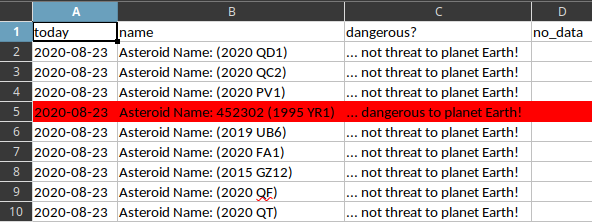
The rows with dangerous asteroids are fill with the red color:
# check asteroids close to planet Earth and add it to file
# import json python package
import json, urllib.request, time

# import openpyxl python package
from openpyxl import Workbook
from openpyxl.styles import PatternFill
# use active worksheet
wb = Workbook()
ws = wb.active

today = time.strftime('%Y-%m-%d', time.gmtime())
print("Time is: " + today)
now = today
# retrieve data about asteroids approaching planet Earth into json format
url = "https://api.nasa.gov/neo/rest/v1/feed?start_date=" + today + "&end_date=" + today + "&api_key=DEMO_KEY"
response = urllib.request.urlopen(url)
result = json.loads(response.read())

print("Now, " + str(result["element_count"]) + " asteroids is close to planet Earth.")
asteroids = result["near_earth_objects"]

no_data = ""
dangerous = ""

ws.append(['today', 'name', 'dangerous?', 'no_data'])
# parsing all the JSON data and add to file
for asteroid in asteroids:
    for field in asteroids[asteroid]:

      try:
        name = "Asteroid Name: " + field["name"]

        if field["is_potentially_hazardous_asteroid"]:   
          dangerous = "... dangerous to planet Earth!"

        else:
          dangerous = "... not threat to planet Earth!"

      except:
        no_data = "no data"
      ws.append([today, name, dangerous, no_data]) 

# create a red patern to fill
redFill = PatternFill(start_color='FFFF0000',
                   end_color='FFFF0000',
                   fill_type='solid')

# check the row with the dangerous asteroid and fill it
for row in ws.rows:
 if row[2].value == "... dangerous to planet Earth!":
  for cell in row:
      cell.fill = redFill

# write all data to file 
wb.save(str(now)+"_asteroids.xlsx")
I run it and result working well:
[mythcat@desk ~]$ python asteroid_data.py 
Time is: 2020-08-23
Now, 9 asteroids is close to planet Earth.
... see the next screenshot:


Saturday, August 22, 2020

Python 3.8.5 : Testing the pyre tool - part 001.

The Pyre is a static analysis tool to detect and prevent security issues in Python code that can be found on the official website.
The Pyre tool supports the Language Server Protocol and has an extension for VSCode.
The team development comes at August 7, 2020, with this intro:
Pyre is a performant type checker for Python. Statically typing what are essentially fully dynamic languages has a long tradition at Facebook. We've done this for PHP with Hack and for Javascript with Flow.
The install is easy to do with pip tool:
[mythcat@desk ~]$ pip install pyre-check
Defaulting to user installation because normal site-packages is not writeable
Collecting pyre-check
  Using cached pyre_check-0.0.52-py3-none-manylinux1_x86_64.whl (22.9 MB)
...
Installing collected packages: pyre-check
Successfully installed pyre-check-0.0.52
If you want to use a virtual environment:
[mythcat@desk ~]$ mkdir my_project && cd my_project
[mythcat@desk my_project]$ python3 -m venv ~/.venvs/venv
[mythcat@desk my_project]$ source ~/.venvs/venv/bin/activate
(venv) [mythcat@desk my_project]$ pip install pyre-check
Collecting pyre-check
...
(venv) [mythcat@desk my_project]$ pyre init
 ƛ Which directory should pyre be initialized in? (Default: `.`): 
(venv) [mythcat@desk my_project]$ cat .pyre_configuration
{
  "binary": "/home/mythcat/.venvs/venv/bin/pyre.bin",
  "source_directories": [
    "."
  ],
  "taint_models_path": "/home/mythcat/.venvs/venv/lib/pyre_check/taint/",
  "typeshed": "/home/mythcat/.venvs/venv/lib/pyre_check/typeshed/"
}
(venv) [mythcat@desk my_project]$ ls .pyre
my_project  pid_files  pyre.stderr
(venv) [mythcat@desk my_project]$ pyre
 ƛ No watchman binary found. 
To enable pyre incremental, you can install watchman: https://facebook.github.io/watchman/docs/install
 ƛ Defaulting to non-incremental check.
 ƛ No type errors found
Let's test with the default example from documentation:
(venv) [mythcat@desk my_project]$ echo "i: int = 'string'" > test.py
(venv) [mythcat@desk my_project]$ pyre
 ƛ No watchman binary found. 
To enable pyre incremental, you can install watchman: https://facebook.github.io/watchman/docs/install
 ƛ Defaulting to non-incremental check.
 ƛ Found 1 type error!
test.py:1:0 Incompatible variable type [9]: i is declared to have type `int` but is used as type `str`.
(venv) [mythcat@desk my_project]$ cat test.py 
i: int = 'string'
You can see is working well and detect the problem.
A short intro can found on the Facebook developers youtube channel:

Saturday, August 15, 2020

Python 3.8.5 : The hashlib python package - part 001.

The tutorial for today is about hashlib python module.
The official webpage comes for this python package has this intro:
This module implements a common interface to many different secure hash and message digest algorithms. Included are the FIPS secure hash algorithms SHA1, SHA224, SHA256, SHA384, and SHA512 (defined in FIPS 180-2) as well as RSA’s MD5 algorithm (defined in Internet RFC 1321).
The example source code to test a simple hash is this:
import hashlib
import os

def file_sha1(filename):
    BUF_SIZE = 65536  # read stuff in 64kb chunks!
    get_sha1 = hashlib.sha1()
    with open(filename, 'rb') as f:
        while True:
            data = f.read(BUF_SIZE)
            if not data:
                break
            get_sha1.update(data)
    return get_sha1.hexdigest()

# I add this comment after first to see the hash difference.
files = [f for f in os.listdir('.') if os.path.isfile(f)]
for f in files:
    h = file_sha1(f)
    print(h) 
Let's test the source code with the default directory and two files.
I run it first with default source code and then I add a comment to test_hash_file.py file.
You can see the hash is changed from b222523567a8a806382b86578717ddbd00e0f4b4 to 2134660551cc67812413a3a75fd12efb05d591ef.
[mythcat@desk Projects_Python]$ ls
test_hash_file.py  test_numpy_001.py
[mythcat@desk Projects_Python]$ python test_hash_file.py 
98b2833527ad3d9fe263542c6aa06c04182d3dfb
b222523567a8a806382b86578717ddbd00e0f4b4
[mythcat@desk Projects_Python]$ python test_hash_file.py 
98b2833527ad3d9fe263542c6aa06c04182d3dfb
2134660551cc67812413a3a75fd12efb05d591ef

Sunday, August 9, 2020

Python 3.8.5 : Pearson Product Moment Correlation with corrcoef from numpy.

The python package named numpy come with corrcoef function to return Pearson product-moment correlation coefficients.
This method has a limitation in that it can compute the correlation matrix between two variables only.
The full name is the Pearson Product Moment Correlation (PPMC).
The PPMC is not able to tell the difference between dependent variables and independent variables.
The documentation about this function can be found here.
More examples of Pearson Correlation can be found on this website.
My example presented in this tutorial, use the random packet to randomly generate integers and then calculate the correlation coefficients.
All of these are calculated five times in a for a cycle and each time the seed parameters are changed randomly.
Each time the correlation matrices are printed and then the random number graphs are displayed.
Let's see the source code:
import random

import numpy as np

nr_integers = 100
size_integers = 100

import matplotlib
import matplotlib.pyplot as plt

# set from 0 to 4 seed for random and show result 
for e in range(5):
    # change random seed
    np.random.seed(e)
    # nr_integers random integers between 0 and size_integers
    x = np.random.randint(0, size_integers, nr_integers)
    # Positive Correlation with some noise created with
    # nr_integers random integers between 0 and size_integers
    positive_y = x + np.random.normal(0, size_integers, nr_integers)
    correlation_positive = np.corrcoef(x, positive_y)
    # show matrix for correlation_positive
    print(correlation_positive)
    # Negative Correlation with same noise created with 
    # nr_integers random integers between 0 and size_integers
    negative_y = 100 - x + np.random.normal(0, size_integers, nr_integers)
    correlation_negative = np.corrcoef(x, negative_y)
    # show matrix for output with plt
    print(correlation_negative)
    # set graphic for plt with two graphics for each output with subplot
    plt.subplot(1, 2, 1)
    plt.scatter(x,positive_y)
    plt.subplot(1, 2, 2)
    plt.scatter(x,negative_y)
    # show the graph 
    plt.show()


Tuesday, August 4, 2020

Python 3.6.9 : My colab tutorials - part 008.

Today I deal with these two python packages named selenium and chromium-chromedriver.
I used selenium to get pieces of information from webpages.
These examples can be found at my GitHub project colab on the notebook named catafest_008.