Using python modules: mayavi and moviepy - part 001.

This is a simple example with two modules named: mayavi and moviepy.
Let's see the introduction of these python modules:
Mayavi2 is a general purpose, cross-platform tool for 3-D scientific data visualization. Its features include:

• Visualization of scalar, vector and tensor data in 2 and 3 dimensions.
• Easy scriptability using Python.
• Easy extendibility via custom sources, modules, and data filters.
• Reading several file formats: VTK (legacy and XML), PLOT3D, etc.
• Saving of visualizations.
• Saving rendered visualization in a variety of image formats.
• Convenient functionality for rapid scientific plotting via mlab

MoviePy is a Python module for video editing, which can be used for basic operations (like cuts, concatenations, title insertions), video compositing (a.k.a. non-linear editing), video processing, or to create advanced effects. It can read and write the most common video formats, including GIF.
The installation with pip3.6 tool:

C:\Python364\Scripts>pip3.6.exe install mayavi
Requirement already satisfied: mayavi in c:\python364\lib\site-packages (4.6.2)
...
C:\Python364\Scripts>pip3.6.exe install moviepy
Collecting moviepy
...
Installing collected packages: tqdm, moviepy
Successfully installed moviepy-0.2.3.5 tqdm-4.28.1

Let's create a simple example with these python modules.
First example:

C:\Python364>python.exe
Python 3.6.4 (v3.6.4:d48eceb, Dec 19 2017, 06:54:40) [MSC v.1900 64 bit (AMD64)]
 on win32
Type "help", "copyright", "credits" or "license" for more information.
>>> import mayavi.mlab as mlab
>>> f = mlab.gcf()
>>> f.scene._lift()
>>>

I choose the most common filter math function: the sinc function, known as sine cardinal:
In signal processing, a sinc filter is an idealized filter that removes all frequency components above a given cutoff frequency, without affecting lower frequencies, and has linear phase response. The filter's impulse response is a sinc function in the time domain, and its frequency response is a rectangular function.
I create the example to show you a sinc function by time.
This is my output (is not the result of the frequency response of the Fourier transform of the rectangular function).

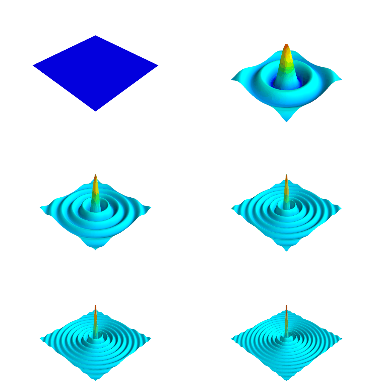
Let's see the source code:

# import python modules
import numpy as np
import mayavi.mlab as mlab
import moviepy.editor as mpy
# duration of the animation in seconds 
duration= 2
# create the grid of points for x and y
x, y = np.mgrid[-30:30:100j, -30:30:100j]
# create the size figure
fig = mlab.figure(size=(640,480), bgcolor=(1,1,1))
# create the plane surface
r = np.sqrt(x**2 + y**2)
# this fix issue https://github.com/enthought/mayavi/issues/702
fig = mlab.gcf()
fig.scene._lift()
# create all frames 
def make_frame(t):
    # clear the area 
    mlab.clf()
    #blend surface by z over time t step is 0.05
    z = np.sin(r*t)/r
    # create surface 
    mlab.surf(z, warp_scale='auto')
    return mlab.screenshot(antialiased=True)
# create animation movie clip
animation = mpy.VideoClip(make_frame,duration=duration)
# write file like a GIF 
animation.write_gif("sinc.gif", fps=20)

Python Qt5 : the most simple QTreeWidget - part 001.

The QTreeWidget is more complex in order to accomplish a simple development issue.
Today, I will show you how is the first step to start it.
This simple example will follow these goals:

• create a simple QTreeWidget;
• use the most simple way to do that;
• do not use the class object;
• show files and folders;

The example do not have any feature for and show my C drive:

• filter, sort and drag and drop;

The result of this example:

Using pytorch - the final of story.

Let's continue our story with the child and the gift.
The child saw the gift and his first thought was the desire to know.
The basic forming unit of a neural network is a perceptron.
He saw that he was not too big and his eyes lit up.
To compute the output will multiply input with respective weights and compare with a threshold value.
Each perceptron also has a bias which can be thought of as how much flexible the perceptron is.
This process is of evolving a perceptron to what a now called an artificial neuron.
The next step is the artificial network and is all artificial neuron and edges between.
He touched him in the corners and put his hand on his surface.
The activation function is mostly used to make a non-linear transformation which allows us to fit nonlinear hypotheses or to estimate the complex functions.
He began to understand that he had a special and complex form.
This artificial network is built from start to end from:

• Input Layer an X as an input matrix;
• Hidden Layers a matrix dot product of input and weights assigned to edges between the input and hidden layer, then add biases of the hidden layer neurons to respective inputs and use this to update all weights at the output and hidden layer to use update biases at the output and hidden layer.
• Output Layer an y as an output matrix;

Without too much thoughts he began to break out of the gift in the order in which he touched it.
This weight and bias of the updating process are known as back propagation.
To computed the output and this process is known as forward propagation.
Several moves were enough to complete the opening of the gift.
He looked and understood that the size of the gift is smaller, but the gift was thankful to him.
This forward and back propagation iteration is known as one training iteration named epoch.
The next example I created from an old example I saw on the internet and is the most simple way to show you the steps from this last part of the story:

##use an neural network in pytorch
import torch

#an input array
X = torch.Tensor([[1,0,1],[0,1,1],[0,1,0]])

#the output
y = torch.Tensor([[1],[1],[0]])

#the Sigmoid Function
def sigmoid (x):
  return 1/(1 + torch.exp(-x))

#the derivative of Sigmoid Function
def derivatives_sigmoid(x):
  return x * (1 - x)

#set the variable initialization
epoch=1000 #training iterations is epoch
lr=0.1 #learning rate value
inputlayer_neurons = X.shape[1] #number of features in data set
hiddenlayer_neurons = 3 #number of hidden layers neurons
output_neurons = 1 #number of neurons at output layer

#weight and bias initialization
wh=torch.randn(inputlayer_neurons, hiddenlayer_neurons).type(torch.FloatTensor)
print("weigt = ", wh)
bh=torch.randn(1, hiddenlayer_neurons).type(torch.FloatTensor)
print("bias = ", bh)
wout=torch.randn(hiddenlayer_neurons, output_neurons)
print("wout = ", wout)
bout=torch.randn(1, output_neurons)
print("bout = ", bout)

for i in range(epoch):

  #Forward Propogation
  hidden_layer_input1 = torch.mm(X, wh)
  hidden_layer_input = hidden_layer_input1 + bh
  hidden_layer_activations = sigmoid(hidden_layer_input)
 
  output_layer_input1 = torch.mm(hidden_layer_activations, wout)
  output_layer_input = output_layer_input1 + bout
  output = sigmoid(output_layer_input1)

  #Backpropagation
  E = y-output
  slope_output_layer = derivatives_sigmoid(output)
  slope_hidden_layer = derivatives_sigmoid(hidden_layer_activations)
  d_output = E * slope_output_layer
  Error_at_hidden_layer = torch.mm(d_output, wout.t())
  d_hiddenlayer = Error_at_hidden_layer * slope_hidden_layer
  wout += torch.mm(hidden_layer_activations.t(), d_output) *lr
  bout += d_output.sum() *lr
  wh += torch.mm(X.t(), d_hiddenlayer) *lr
  bh += d_output.sum() *lr
 
print('actual :\n', y, '\n')
print('predicted :\n', output)

The result is for 100 and 1000 epoch value and show us how close is the actual input (1,1,0) to the predicted results.
See also the weight and bias initialization of the artificial network is created random by torch.randn.
If I added this in my story it would sound like this:
The child's thoughts began to flinch in wanting to finish faster and find the gift.

C:\Python364>python.exe pytorch_test_002.py
weigt =  tensor([[-0.9364,  0.4214,  0.2473],
        [-1.0382,  2.0838, -1.2670],
        [ 1.2821, -0.7776, -1.8969]])
bias =  tensor([[-0.3604, -0.8943,  0.3786]])
wout =  tensor([[-0.5408],
        [ 1.3174],
        [-0.7556]])
bout =  tensor([[-0.4228]])
actual :
 tensor([[1.],
        [1.],
        [0.]])

predicted :
 tensor([[0.5903],
        [0.6910],
        [0.6168]])

C:\Python364>python.exe pytorch_test_002.py
weigt =  tensor([[ 1.2993,  1.5142, -1.6325],
        [ 0.0621, -0.5370,  0.1480],
        [ 1.5673, -0.2273, -0.3698]])
bias =  tensor([[-2.0730, -1.2494,  0.2484]])
wout =  tensor([[ 0.6642],
        [ 1.6692],
        [-0.4087]])
bout =  tensor([[0.3340]])
actual :
 tensor([[1.],
        [1.],
        [0.]])

predicted :
 tensor([[0.9417],
        [0.8510],
        [0.2364]])

Python Qt5 : simple draw with QPainter.

Using the QPainter is more complex than a simple example.
I try to create a simple example in order to have a good look at how can be used.
The main goal was to understand how can have the basic elements of QPainter.
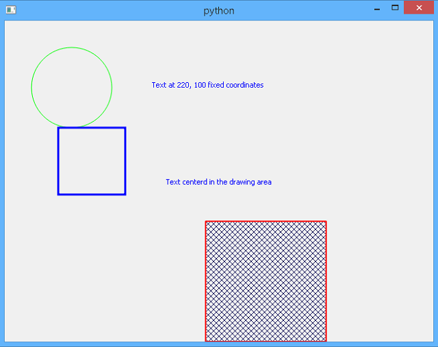
The result of my example is this:

Here is my example with all commented lines for a good approach:

import sys 
from PyQt5 import QtGui, QtWidgets 
from PyQt5.QtGui import QPainter, QBrush, QColor
from PyQt5.QtCore import Qt, QPoint 
class My_QPainter(QtWidgets.QWidget): 
    def paintEvent(self, event): 
        # create custom QPainter
        my_painter = QtGui.QPainter() 
        # start and set my_painter
        my_painter.begin(self) 
        my_painter.setRenderHint(my_painter.TextAntialiasing, True)
        my_painter.setRenderHint(my_painter.Antialiasing, True)
        #set color for pen by RGB
        my_painter.setPen(QtGui.QColor(0,0,255)) 
        # draw a text on fixed coordinates
        my_painter.drawText(220,100, "Text at 220, 100 fixed coordinates") 
        # draw a text in the centre of my_painter   
        my_painter.drawText(event.rect(), Qt.AlignCenter, "Text centerd in the drawing area") 
        #set color for pen by Qt color  
        my_painter.setPen(QtGui.QPen(Qt.green, 1)) 
        # draw a ellipse
        my_painter.drawEllipse(QPoint(100,100),60,60) 
        # set color for pen by property
        my_painter.setPen(QtGui.QPen(Qt.blue, 3, join = Qt.MiterJoin)) 
        # draw a rectangle
        my_painter.drawRect(80,160,100,100) 
        # set color for pen by Qt color 
        my_painter.setPen(QtGui.QPen(Qt.red, 2))
        # set brush 
        my_brush = QBrush(QColor(33, 33, 100, 255), Qt.DiagCrossPattern)
        my_painter.setBrush(my_brush)
        # draw a rectangle and fill with the brush 
        my_painter.drawRect(300, 300,180, 180)
        my_painter.end() 
# create application  
app = QtWidgets.QApplication(sys.argv) 
# create the window application from class
window = My_QPainter() 
# show the window
window.show() 
# default exit 
sys.exit(app.exec_())

Python 3.6.4 : Learning OpenCV - centroids.

Today I was a little lazy.
I studied a little on the internet.
The last aspect was related to centroids.
An example I studied before TV news was from this webpage.
About centroid you can read here.
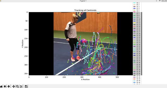
The result of the source code from a video with Simona Halep.